TẠP CHÍ: KINH TẾ & QTKD, TRƯỜNG ĐH KINH TẾ & QTKD THÁI NGUYÊN; SỐ 04 NĂM 2012

Cù Phúc Thành

Viện Nghiên cứu Kinh tế & PTNNL, Trường ĐH Kinh tế & QTKD Thái Nguyên

ABSTRACT

Upper catchments of the Mountainous Areas of Northern Vietnam are encountering a serious dual problem of poverty and natural resource degradation. To earn a living farming populations there just perform quasi-subsistent agricultural practices that depend heavily on natural resources. Unfortunately, those practices turn back to be the main agent that severely deteriorates those very resources. No doubt, there must be research to search for solutions in order to overcome the problem. Of cause, research will obtain better results if helped with a powerful tool, methodologically. Among modern tools, Farm Household Model using Linear Programming shows reliable and broad-used. This study was an effort to construct a linearly programmed model as functional as possible in simulating the farming households in the Mountainous Areas of Northern Vietnam to facilitate studies upon request.                     

Key Words: Subsistent Agriculture, Farm Household Model, Linear Programming, Mountainous Areas of Northern Vietnam

 

1            INTRODUCTION

For centuries, ethnic minority groups used to move place to place around upper catchments of the Red river basin, burning down forest at mountain sides and sowing crops there till the soil got exhausted. This incidence has already degraded natural resources in large scale in the Mountainous Areas of Northern Vietnam while not helped inhabitants escape poverty. Today, there are blatant evidences proving the picture even gets gloomier. With rapidly marginalized population, with hard farming conditions resulted from high altitude and steep topography, with low agricultural productivity the vicious circle of poverty and resource degradation seems to be captured in dilemma eternally. Clearly, there must be action to respond to the question. But to effectively hit the target, action must be over-brooded from research which will be double-strengthened if equipped with a mighty tool. Among the best ones, a model of farmers’ behaviors in decision making for their productions shows itself a powerful and multipurpose tool. There has not been a wide selection of models of that type for the Mountainous Areas of Northern Vietnam yet, and that is why this study came to existence.

In fact, this paper is adapted from a report of an international joint project initiated and presided by International Rice Research Institute (IRRI). Abbreviated PN11, carried out in the second half of the decade of 2000s with the research sphere covering mountainous parts of Mianma, Thailand, Lao and Vietnam, the full name of the project is Rice Landscape Management for Raising Water Productivity, Conserving Resources, and Improving Livelihoods in Upper Catchments of the Mekong and Red River Basins. In Vietnam, among the studies conducted, there was one of constructing a Farm Household Model of farming households in the Mountainous Areas of Northern Vietnam, which was directly conducted by a group of researchers comprising of PhD. Damien Jourdain – a scientist seconded to IRRI from Center of International Cooperation in Agronomic Research for Development (CIRAD, France) who presided the project implementation in Vietnam, Dang Dinh Quang – a researcher from Northern Mountainous Agriculture and Forestry Science Institute (NOMAFSI, Vietnam), Esther Boere and Cu Phuc Thanh – students at Master level respectively from Wageningen (Netherland) and Thainguyen University of Economics and Business Administration (TUEBA, Vietnam). 

The main agent that causes the vicious circle in upper catchments of the Red is the way farming populations there conduct their livelihood activities. Thus, to solve the problem, in the first place we should get comprehension of that very way. And that very way has persisted long and repeatedly, it will be ideal if we can catch the form of its behavior because on that basis we can anticipate what farmers will do in a given production context and hence can drive that doing to an objective positive on resource conservative and livelihood improving aspects, namely if we can model farmers’ production behaviors. 

Because in one hand, a farmer’s production is always steered to an objective that is predestined by their desire to maximize their possible benefits and well-being but, in the other hand that production is always bounded by a set of constraints on resources that farmer can have available, an optimizing model is worldwide recommended. So, the objective of this study is to construct an optimizing model that can as precisely as possibly simulate the behaviors in selecting livelihood strategies of farming households in the Mountainous Areas of Northern Vietnam to make provided a strong tool for further studies directly aiming at searching for solutions for the problem in the regions.    

2            METHODOLOGY

2.1         Linear Programming

Methodologically, there is a wide range of optimizing modeling styles differentiated from one another depending on what algorithm used to develop them. Among styles, Farm Household Model (FHM) using Linear Programming (LP) is so prevailingly used for its high accuracy, effectiveness, multipurpose use, flexibility and simplicity. Thus, we used it in this study.

Algebraically, the methodology of LP can simply be stated in the three following equations.

 MaxZ = Σc_jX_j                     j = 1 to  n                       (1)

Σa_ijX_j  <  b_i                          i = 1 to m                       (2)

and:    

        X_j  > 0                           j = 1 to n                       (3)

Where (1) describes the objective function with Z symbolizing the goal for which the household conducts their livelihood plan; Z is usually profit, but in many developing countries where subsistent farming still exists, it is utility or other nonprofit purposes instead; Conventionally, Z is termed ‘Gross Margin’ (GM); Also in Equation (1), j depicts livelihood activities the household can possibly choose to achieve their goal; These activities are mainly of crops or livestock, but in case the household does conduct a non-agricultural activity as a part of their livelihood means, we then have to fully take it into account for the model not to be out of reality because it will compete with farming ones over constrained resources; The note of ‘j = 1 to n’ implies in total there are n activities available to the household (implicitly, n > 0 and of integer); X stands for the level of an activity selected by the household in their optimized plan, so X_j means activity j is selected at level X; X is quantified in some measuring system, for example ha or ton…;  C_j is the quantity of GM yielded from one unit of j. With decoding for all the symbols, Equation (1) implies the household desires to maximize their total GM.

In the generic Equation (2), i is representative for resources required for activities conducted, for example land, labor, water or cash...; a_ij means producing one unit of j requires a units of i; In total, the household has m resources (m > 0 and of integer, too); Because the household cannot have infinitive in amount of any resource, at the same time in the short-run they cannot change the amounts of all their resources, bi implicitly means the household only has resource i steadily (or fixedly) at level b. So, (2) abstracts all the constraints the household has to face. It speeches that the total use of any resource for all activities selected for the optimized plan mustn’t exceed the fixed quantity of that resource.

Of cause it would be nonsense to suppose the household may select an activity at a level below zero (3).

In the real world, Equations (1) to (3) describe the household desires to maximize their well-being by conducting a livelihood strategy. Nevertheless, they cannot do that at will but under the constraint of a set of resource limitations. Consequently, they try to optimize their goal with what they have available in hand.

The Equations are a problem the farmer solves by intuition but we have to do by reasoning. From our point of view, (1), (2), (3) are equations; X_j are variables we need to find out; c_j, a_ij, b_i are given parameters. In terms of LP, conventionally, (1), (2), (3) are still called equations; j are called activities; X_j exogenous or endogenous variables; c_j, a_ij, b_i given technical coefficients.

Despite its simple form, it is extremely complicated to solve the problem of LP, mathematically. It is so difficult that it was long time before the solution was found out and that is why a Nobel prize was given to Danzig for his discover of simplex algorithm. What is more, despite the clear solving principles, the procedures to solve an LP problem by simplex algorithm are still so complicated and painstaking that it was rarely applied in research in the recent past. Fortunately, with the computer development, now that difficulty is overcome and LP is used worldwide. Again, despite the helpfulness of the computer, LP application remains such hard work, economically as well as technically, that skilled modelers are not of plenty. In this study, we will solve our FHM problem on the platform of advanced computer software GAMS.

2.2         Household survey

The survey was conducted in Vanchan district, Yenbai province, Vietnam. Topographically, anthropologically, agro-ecologically and socio-economically, Vanchan is a place typical for the Mountainous Areas of Northern Vietnam. We decided to get a sample of 45 typical households. Within the district, four villages were adopted to pick out the sample elements. They were Pangcang in Suoigiang commune, Namchau in Nambung commune, Giangcai in Namlanh commune and Bantun in Tule commune.

With the help of a well designed semi-structured questionnaire, each surveyed household was interviewed in three rounds each of 1.5 to 2 hours. The gathered information was then stored in Microsoft Access Database and made available upon request. For each type of households, a typical one was elicited to model on GAMS platform. 

3            RESEARCH RESULTS

3.1         Resources of households

Households are differentiated in having resources hence to model their productions a typology categorizing them into different groups according to their quantity levels of resources is crucial. In this study we used a typology of households in the Mountainous Areas of Northern Vietnam, which is also a study of PN11, carried out just before our study, conducted by Damien Jourdain, Do Anh Tai, Dang Dinh Quang and Tran Pham Van Cuong. With certain adjustments due to new information gathered from our survey, we defined 6 household groups, symbolized WSLS, WSLR, OFFW, TERLAB, PARI, TERUPL with resource circumstances shown in Table 1.

Table 1: Resources of household groups

Variable	G5 WSLS	G2 WSLR	G6 OFFW	G3 TERLAB	G4 TERUPL	G1 PARI
Household size (person)	4	5	7	8	6	6
Family workforce (worker)	2	2	5	5	3.5	3.5
Lowland irrigated in 2 seasons (m2)	0	0	200	200	100	1500
Lowland irrigated in 1 seasons (m2)	0	0	1500	250	250	3000
Terraces land irrigated in 2 seasons (m2)	0	0	0	300	1000	0
Terraces land irrigated in 1 seasons (m2)	200	500	800	2100	3000	0
Sloping land for dry crops (m2)	6500	14000	7800	8000	16000	15000
Highland for perennial crops (m2)	600	6000	200	9000	5000	4500

The main resources of farmers in the Mountainous Areas of Northern Vietnam are just land and labor. Due to topography, cultivated crops and irrigating status, land was sorted into 6 types, called ‘zones’ in this study.

3.2         Model construction

3.2.1      Activities

The chief activities of the model are cropping activities in cropping systems available in the regions. The most important crop is always irrigated rice. Upland rice, maize, cassava, batata… are also common. Perennial crops are Suoigiang tea, cardamom and cinnemon. Apart from farming, households do sell out or buy in labor and thus labor transaction is integrated in the model as activities, too. Apart, some other livelihood conducts are also incorporated.

3.2.2      Variables

Variables are levels of activities selected by the household in their optimized plan. The main variables are areas of selected cropping systems in m², the amount of labor bought in or sold out.

3.2.3      Periods to model

An FHM will be out of reality if it ignores the fact that households apportion their fixed resources differently to different periods in the production year. In this study, monitoring the common pattern of cropping calendars we divided the production year in the Mountainous Areas of Northern Vietnam into 7 periods with different lengths to model.

3.2.4      Technical coefficients

Technical coefficients of the model are input requirements, yields of crops, input and output prices... These coefficients were elicited from our survey. 

3.2.5      Constraints

3.2.5.1.     Land constraints

                ∑_cX(c,z) < AREA(z)                                                                                            (4)              

Where X(c,z) is the chosen level in m² for cropping system c in zone z and AREA(z) is the area the household has available in that zone.

3.2.5.2      Labor constraints

∑_{c, z}X(c,z) * LABREQ(c,z,t) + LIN(t) < FARMLAB(t) + LOUT(t)                      (5)

LIN(t) < FARMLAB(t) * sLIMBUYLAB(f)                                                          (6)

LOUT(t) < FARMLAB(t) * sLIMSALAB(f)                                                         (7)

Here

• t denotes the periods in the year categorized from T1 to T7  
• f indexes the groups (or types) of households, running from G1 to G6
• LABREQ(c,z,t) stands for the labor requirement of 1 ha of cropping system c in zone z and period t
• FARMLAB(t) is the household labor available in period t
• LIN(t) is the outside labor bought by the household in period t
• LOUT(t) is the household labor apportioned to off-farm activities in period t
• sLIMBUYLAB(f) represents the labor employment limitation of household group f
• sLIMSALAB(f) denotes the upper bound of off-farm labor of group f

The labor available of each group f in period t is calculated by the product of the workforce of that group and the number of working days available in period t.

FARMLAB(t) = WORKFORCE(f) * WRKNGDAYAVAIL(t)                                                  (8)

WORKFORCE(f) symbolizes the number of regular workers of household group f.

3.2.5.3      Product constraints

QBEG(p,t) + QPROD(p,t) + QBUY(p,t) - QCONS(p,t) - QSALE(p,t) = QEND(p,t)            (9)

The notation is given as the followings:

• QBEG(p,t) is the stock of crop p at the beginning of period t
• PROD(p,t), QBUY(p,t), QCONS(p,t) and QSALE(p,t) are the quantities of crop p the household produces, buys, consumes and sells in period t, respectively
• QEND(p,t) is the stock of crop p left at the end of period t

Interviews revealed households only need to buy staples, especially rice for their own consumption and only in case they come across a shortage. However, when they need staples, they cannot purchase them at will. Here market constraint gives effect again: the household can only buy an amount in some ratio to their sufficiency need. The ratio depends on which group the household belongs to, too.  

QBUY(p,t) < QCONS(p,t) * BUYCOEF(f)                                                       (10)

Here BUYCOEF (f) is the coefficient of buying ratio of group f.

Equation 6.6 only describes the product relationships within one period while Equation 6.8 does the relation between periods by means of product transfers. The ending stock of a crop, by transferring, becomes the beginning stock of that crop in the next period with a little reduction in amount due to storage loss.   

QBEG(p,t+1) = QEND(p,t) * cLOSS(p)                                                          (11)

Here: t+1 index the period next to t, and cLOSS(p): the remaining ratio after storage loss, estimated at 99%. Of cause T1 is regarded the next period of T7, conventionally.

To be alert against risks of poor harvests, to serve habitual appetites, to feed domestic animals, to self-solve the problem of redundant labor, for needs in cash and brewery…, dependent on the type of the household, crop diversification is conducted. Algebraically, the crop diversification can be described in Equations 6.9 and 6.10.

∑_tQPROD(ca,t) > CASSDIVERSCOEF(f) * ∑_tQPROD(ma,t)                                              (12)

∑_tQPROD(sp,t) > SPDIVERSCOEF(f) * ∑_tQPROD(ca,t)                                                    (13)

With QPROD(ma,t), QPROD(ca,t), QPROD(sp,t): the quantities of maize, cassava and batata produced in period t respectively, and CASSDIVERSCOEF(f), SPDIVERSCOEF(f): the ratios of cassava to maize and batata to cassava of group f.

The quantity of a product itself depends on the area and the yield of the relating crop. This relation is caught in Equation 6.11 below.

QPROD(p,t) = ∑_{c, z}X(c,z) * YIELD(c,p,z,t)                                                                           (14)

Here YIELD(c,p,z,t) is the quantity of crop p yielded by 1 ha of system c in zone z and period t.

3.2.5.4      Budget constraints                

CASHBEG(t) - LIVING(t) - ∑_pQBUY(p,t) * sPRICE(p) *

(1 + tcc) + ∑_pQSALE(p,t) * sPRICE(p) + LOUT(t) *

LPRICE * (1 - tcl) - LIN(t).LPRICE * (1 + tcl) -

∑_{c, z, t, i}INPUT(c,i,t) * INPPRICE(i) * X(c,z,t) + BORROW(t) -

BORROW(t - 1) * (1 + sINT) = CASHEND(t)                                                                        (15)

In this equation:

• CASHBEG(t) is the cash available of the household at the beginning of period t
• LIVING(t) is the living expenses of the household in period t
• sPRICE(p) is the household selling price of crop p
• LPRICE is the average labor price, estimated at 50,000 VND/day (equivalent to 2.5 USD/day in 2009)
• INPUT(c,i,t) is the amount of input i required by 1 ha of system c in period t
• INPPRICE(i) is the price of input i
• X(c,z,t) is the area of system c in zone z in period t
• BORROW(t) is the money borrowed in period t
• BORROW(t-1) is the money borrowed in the previous period and paid back with an interest in period t
• CASHEND(t) is the cash left over at the end of period t
• tcc is the rate of ‘transaction costs’ in product market, representing the gap between the farm-gate and market prices of the crop, estimated at 20% of the farm-gate price 
• tcl is the rate of ‘transaction costs’ in labor market, implying the extra costs both the employer and employee have to be charged, estimated at 20% of the average labor price
• sINT is the average interest rate, calculated at 0.03

One of the factors that differentiate households from one another is their accessibility to product market graded by the ratio of the real farm-gate price at which the household sells a product to the average farm-gate price. This differentiation is taken into the model by

sPRICE(p) = AVRPRICE(p) * MARKETCOEF(f)                                                          (16)

With AVRPRICE(p) denoting the average farm-gate price of crop p and MARKETCOEF(f): the ratio of the actual farm-gate price at which the household can sell the product to the average farm-gate level.

Similar to the product balances, each CASHEND transforms itself to the CASHBEG of the next period, of cause no storage loss existing in this case and again T7 previous to T1.

CASHEND(t) = CASHBEG(t+1)                                                                                    (17)

The next algebraic statement of the model is constraints on capabilities of borrowing money of households. In period t, if in case, the household can only borrow an amount of money at maximum equal to the total value of all their existing crops expected to harvest in the next period.

BORROW(t) < ∑QPROD(p,t+1) * sPRICE(p)                                                               (18)

Here QPROD (p,t+1) is the output of crop p, expected to obtain in period t+1.

3.2.5.5      Consumption constraints

RICECONS(t) + RICESHORT(t) > RICEMINEED(t)                                                              (19)

RICECONS(t) > 0.45 * RICEMINEED(t)                                                                                 (20)

MAIZECONS(t) > 2 * RICESHORT(t) + MAIZESHORT(t)                                                     (21)

CASSCONS(t) > 2 * MAIZESHORT(t)                                                                                   (22)

Notation:

• RICECONS(t): the quantity of rice the household actually consume in period t
• RICEMINEED(t): the quantity of rice the household need in the whole period t on the basis of 0.5 kg/person/day
• RICESHORT(t): the rice shortage in period t
• MAIZECONS(t): the quantity of maize consumed by the household in period t
• MAIZESHORT(t): the maize shortage in period t
• CASSCONS(t): the quantity of cassava consumed in period t. Cassava is assumed no shortage for its easy availability

3.2.6       Objective function

Unlike farms in developed countries, farming households in the Mountainous Areas of Northern Vietnam maximize not income but utility decodable in terms of money.

CASHEND(T6) - BORROW(T6) * wBORR –

∑_tRICESHORT(t) * wRSHORT = UTIL                                                                       (23)

Where:

• UTIL: the optimized variable representing utility
• wBORR: the linear weight of the loss function of failing to meet minimum cash need of the household
• wRSHORT: the linear weight of the loss function of rice shortage

3.2.7      Model Calibration

All the six groups of households were calibrated with also six calibrated coefficients or parameters: limitations in buying products and labor, ratios of the productions of cassava and batata, and capability of selling products at higher prices.

3.3         Model validation

After constructed and calibrated, the model works well and perfectly simulates the livelihood strategies of the household groups. The comparisons between data from the model and those from the survey are displayed in Table 2.

Table 2: Household livelihood strategies - Model vs Survey

                 

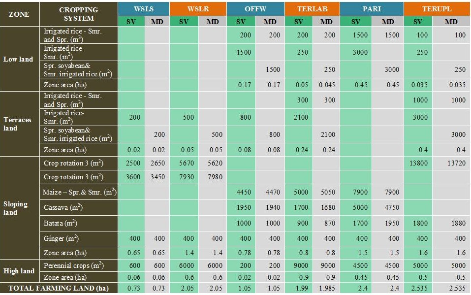
Notes:   SV = data from survey; MD = data from model; Spr. = Spring; Smr. = Summer; Crop rotation 3 = Crop rotation in 10 years: 3 years of upland rice + 2 years of cassava + 3 years of maize + 2 years of fallow; Crop rotation 4 = Crop rotation in 6 years: 2 years of upland rice + 2 years of cassava + 2 years of fallow

4          CONCLUSION

The survey and the model agree that in general farming households in the Mountainous Areas of Northern Vietnam are very poor with modest irrigated land - the resource decisive to their well-being. With minor differences between the survey and the model, the validation affirms the model can simulate livelihood strategies of farming households in the regions exactly. This proves that the model can be used as a strong tool in many fields of concerning research and real-world policy making. In fact, we have applied it in a lot of further research on resource conservation and livelihood improvement and it showed very useful and reliable. However, because the socio-economic contexts of farming populations in upper catchments of the Red river do change with their resources becoming different the model needs to be regularly updated. Last but not least, our model was constructed just on single-horizon basis leaving more advanced models to more skilled modelers.

 

REFRENCES

Affholder F., Jourdain D., Quang D. D., Tuong T. P., Morize M. & Ricome A. (2010). Constraints to farmers' adoption of direct-seeding mulch-based cropping systems: A farm scale modeling approach applied to the mountainous slopes of Vietnam. Agricultural Systems, 103(1), 51-62.

Damien Jourdain, Dang Dinh Quang, Esther Boere, Cu Phuc Thanh (2010). Trade-off analysis in the use of water: farm and small catchment simulations,PN11 Vietnam Reports, Hanoi.

Damien Jourdain, Pham Van Cuong, Do Anh Tai, Dang Dinh Quang (2009). Access to water and livelihood strategies: a typology of agricultural households in Nam Bung commune, Yen Bai Province, Vietnam, Rice Landscape Management for Raising Water Productivity, Conserving Resources, and Improving Livelihoods in Upper Catchments of the Mekong and Red River Basins, PN11 Vietnam Reports: No. 2009-1, Hanoi.

Damien Jourdain, Pham Van Cuong, Do Anh Tai, Dang Dinh Quang (2009). Access to water and livelihood strategies: a typology of agricultural households in Suoi Giang commune, Yen Bai Province, Vietnam, Rice Landscape Management for Raising Water Productivity, Conserving Resources, and Improving Livelihoods in Upper Catchments of the Mekong and Red River Basins, PN11 Vietnam Reports: No. 2009-1, Hanoi.

Cu Phuc Thanh (2011). Impacts of Pricing Policy on Natural Resources and Livelihoods of Farming Populations in Vanchan District, Yenbai Province, Vietnam, Msc. Thesis of Agricultural Economics.

Hazell P. B. R. & Norton R. D. (1986). Mathematical programming for economic analysis in agriculture. Macmillan Publishing Company, New York.

Rosenthal R. E.. GAMS: a user's guide. GAMS Development Corporation, Washington, D.C (2007).